Often times engineering teams face performance or memory issues caused by database requests. I’m a Ruby engineer, and Ruby is known as a not most performant programming language, so sometimes people believe that rewriting the app with something faster (like Go) will solve their performance issues. If the database is the bottleneck—a complete rewrite won’t help!
In this article we will learn how to move complex calculations from the application to the database level focusing on window functions.
Preparing our lab
In our examples we’ll use a sample database from postgresqltutorial.com. This is how you can get it using the command–line–fu (I’m assuming that you already have PostgreSQL installed, please note that I used 14.2 to prepare these snippets):
createdb dvdrental && \
  curl -o dvdrental.zip 'https://www.postgresqltutorial.com/wp-content/uploads/2019/05/dvdrental.zip' && \
  unzip ./dvdrental.zip && \
  pg_restore -U postgres -d dvdrental ./dvdrental.tar && \
  rm dvdrental.tar
Here is a table diagram:
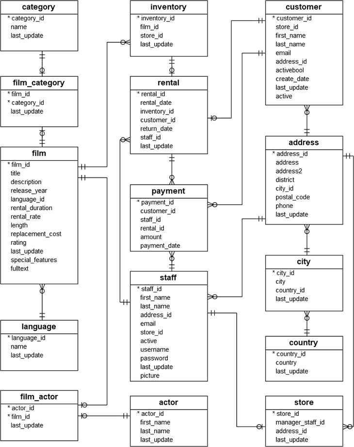
There are a lot of tables, but we will only use a half of them. Films are stored in the film table, and we will only use title and film_id (a primary key). All possible film categories are stored in the category table and, because films can have more than one category, there is a many–to–many table film_category to represent this relation.
Individual DVDs are stored in the inventory table, which can be connected with films using film_id. When customer takes a DVD from one of our shops, a rental row is created. Along with inventory_id, rental has start and end dates as well as the connection with payment table.
Ordering more DVDs
Let’s try to build something real! Our first task is to get a list of most rented films in each category: we need to understand what people like more and order more disks. We want to see something like this:
1   Action      Rugrats Shakespeare
2   Action      Handicap Boondock
3   Action      Primary Glass
1   Animation   Juggler Hardly
2   Animation   Dogma Family
3   Animation   Storm Happiness
Let’s try to build that list using SQL query:
WITH film_with_rental_count AS (
  SELECT film.*, COUNT(rental.*) AS rental_count
  FROM film
  JOIN inventory USING (film_id)
  JOIN rental USING (inventory_id)
  GROUP BY film.film_id
)
SELECT
  category.name,
  film_with_rental_count.title,
  film_with_rental_count.rental_count
FROM film_with_rental_count
JOIN film_category USING (film_id)
JOIN category USING (category_id)
ORDER BY category.name, rental_count DESC;
Firstly, we create a common table expression (or CTE) to build a list of films with rental counts:
SELECT film.*, COUNT(rental.*) AS rental_count
FROM film
JOIN inventory USING (film_id)
JOIN rental USING (inventory_id)
GROUP BY film.film_id
…after that, we order this list by category name and rentals count:
SELECT
  category.name,
  film_with_rental_count.title,
  film_with_rental_count.rental_count
FROM film_with_rental_count
JOIN film_category USING (film_id)
JOIN category USING (category_id)
ORDER BY category.name, rental_count DESC;
…and here is the result we get (the response is rather huge, so it’s just a part of it):
┌─────────────┬─────────────────────────────┬──────────────┐
│    name     │            title            │ rental_count │
├─────────────┼─────────────────────────────┼──────────────┤
│ Action      │ Rugrats Shakespeare         │           30 │
│ Action      │ Suspects Quills             │           30 │
│ Action      │ Handicap Boondock           │           28 │
│ Action      │ Trip Newton                 │           28 │
│ Action      │ Story Side                  │           28 │
│ Action      │ Primary Glass               │           27 │
│ Action      │ Fantasy Troopers            │           26 │
                            ...
└─────────────┴─────────────────────────────┴──────────────┘
Looks good! We can group this dataset by name and iterate over it using our favourite programming language to assign positions. However, it would be nice to get the position of the film right from the PSQL. Also, please note that “Rugrats Shakespeare” and “Suspects Quills” share the first place, should they share a first place or not?
We need a way to assign the position of each film in each category according to its rental_count, so meet window functions.
Window function allows us to calculate the value that is related to the current row, but also using the data from others. It’s very similar to the regular aggregate functions (moreover, many aggregate functions can be used as window ones), but rows stay separate instead of getting grouped. The idea is that we specify the groups of rows we want to use and how to order them, then specify what we need to calculate, and, when calculation is finished, we forget about this temporary grouping. Check out this tutorial for more details.
We are going to use the function called DENSE_RANK, that adds a rank to each partition:
WITH film_with_rental_count AS (
  SELECT film.*, COUNT(rental.*) AS rental_count
  FROM film
  JOIN inventory USING (film_id)
  JOIN rental USING (inventory_id)
  GROUP BY film.film_id
)
SELECT
  category.name,
  DENSE_RANK() OVER (
    PARTITION BY category.category_id
    ORDER BY film_with_rental_count.rental_count DESC
  ) AS category_rank,
  film_with_rental_count.title,
  film_with_rental_count.rental_count
FROM film_with_rental_count
JOIN film_category USING (film_id)
JOIN category USING (category_id)
ORDER BY category.name;
This is the result we’ll get:
┌─────────────┬───────────────┬─────────────────────────────┬──────────────┐
│    name     │ category_rank │            title            │ rental_count │
├─────────────┼───────────────┼─────────────────────────────┼──────────────┤
│ Action      │             1 │ Rugrats Shakespeare         │           30 │
│ Action      │             1 │ Suspects Quills             │           30 │
│ Action      │             2 │ Handicap Boondock           │           28 │
│ Action      │             2 │ Trip Newton                 │           28 │
│ Action      │             2 │ Story Side                  │           28 │
│ Action      │             3 │ Primary Glass               │           27 │
│ Action      │             4 │ Fantasy Troopers            │           26 │
│ Action      │             4 │ Stagecoach Armageddon       │           26 │
│ Action      │             5 │ Hills Neighbors             │           25 │
│ Action      │             5 │ Clueless Bucket             │           25 │
                                  ...
│ Animation   │             1 │ Juggler Hardly              │           32 │
│ Animation   │             2 │ Dogma Family                │           30 │
│ Animation   │             3 │ Storm Happiness             │           29 │
│ Animation   │             4 │ Blackout Private            │           27 │
│ Animation   │             4 │ Forrester Comancheros       │           27 │
                                  ...
└─────────────┴───────────────┴─────────────────────────────┴──────────────┘
What did we change in the query? Added the DENSE_RANK call, which groups films by category, orders them by rental_count and adds to the result, making films with the same rental count share the same position:
DENSE_RANK() OVER (
  PARTITION BY category.category_id
  ORDER BY film_with_rental_count.rental_count DESC
) AS category_rank
Note that we do not need to order films by rental_count on the top level—they are already ordered thanks to the window function.
Is it possible to skip next position when two films share the same position, e.g. ranks can be 1, 2, 3 or 1, 1, 3 but not 1, 1, 2? Sure, use RANK:
WITH film_with_rental_count AS (
  SELECT film.*, COUNT(rental.*) AS rental_count
  FROM film
  JOIN inventory USING (film_id)
  JOIN rental USING (inventory_id)
  GROUP BY film.film_id
)
SELECT
  category.name,
  RANK() OVER (
    PARTITION BY category.category_id
    ORDER BY film_with_rental_count.rental_count DESC
  ) AS category_rank,
  film_with_rental_count.title,
  film_with_rental_count.rental_count
FROM film_with_rental_count
JOIN film_category USING (film_id)
JOIN category USING (category_id)
ORDER BY category.name;
In order to prepare enough DVDs, we need to know most popular films in each category. Let’s take 3 first films, how can we do that?
WITH
  film_with_rental_count AS (
    SELECT film.*, COUNT(rental.*) AS rental_count
    FROM film
    JOIN inventory USING (film_id)
    JOIN rental USING (inventory_id)
    GROUP BY film.film_id
  ),
  category_rankings AS (
    SELECT
      category.name AS category_name,
      ROW_NUMBER() OVER (
        PARTITION BY category.category_id
        ORDER BY film_with_rental_count.rental_count DESC
      ) AS category_rank,
      film_with_rental_count.title AS film_title,
      film_with_rental_count.rental_count AS rental_count
    FROM film_with_rental_count
    JOIN film_category USING (film_id)
    JOIN category USING (category_id)
  )
SELECT *
FROM category_rankings
WHERE category_rank <= 3
ORDER BY category_name;
Window functions cannot be used inside WHERE clause (because they are performed on the result set), so we have to add another CTE called category_rankings. This CTE is used to filter all films that have row number bigger than 3. Also, since we need 3 films, we cannot use RANK or DENSE_RANK, so we replaced them with ROW_NUMBER. This is the result:
┌───────────────┬───────────────┬──────────────────────┬──────────────┐
│ category_name │ category_rank │      film_title      │ rental_count │
├───────────────┼───────────────┼──────────────────────┼──────────────┤
│ Action        │             1 │ Rugrats Shakespeare  │           30 │
│ Action        │             2 │ Suspects Quills      │           30 │
│ Action        │             3 │ Handicap Boondock    │           28 │
│ Animation     │             1 │ Juggler Hardly       │           32 │
│ Animation     │             2 │ Dogma Family         │           30 │
│ Animation     │             3 │ Storm Happiness      │           29 │
│ Children      │             1 │ Robbers Joon         │           31 │
│ Children      │             2 │ Idols Snatchers      │           30 │
│ Children      │             3 │ Sweethearts Suspects │           29 │
│ Classics      │             1 │ Timberland Sky       │           31 │
│ Classics      │             2 │ Frost Head           │           30 │
│ Classics      │             3 │ Voyage Legally       │           28 │
│ Comedy        │             1 │ Zorro Ark            │           31 │
│ Comedy        │             2 │ Cat Coneheads        │           30 │
│ Comedy        │             3 │ Closer Bang          │           28 │
                               ...
└───────────────┴───────────────┴──────────────────────┴──────────────┘
Let’s try all three functions alltogether to see the difference:
WITH film_with_rental_count AS (
  SELECT film.*, COUNT(rental.*) AS rental_count
  FROM film
  JOIN inventory USING (film_id)
  JOIN rental USING (inventory_id)
  GROUP BY film.film_id
)
SELECT
  category.name,
  ROW_NUMBER() OVER w AS row_number,
  DENSE_RANK() OVER w AS dense_rank,
  RANK() OVER w AS rank,
  film_with_rental_count.title,
  film_with_rental_count.rental_count
FROM film_with_rental_count
JOIN film_category USING (film_id)
JOIN category USING (category_id)
WINDOW w AS (
  PARTITION BY category.category_id
  ORDER BY film_with_rental_count.rental_count DESC
)
ORDER BY category.name;
Oh, wait, what’s the WINDOW? In cases when you have to copy and paste the same expression for multiple OVER you can extract it to the named WINDOW and reuse it! And now, the result of the execution:
┌──────────┬────────────┬────────────┬──────┬──────────────────────┬──────────────┐
│   name   │ row_number │ dense_rank │ rank │        title         │ rental_count │
├──────────┼────────────┼────────────┼──────┼──────────────────────┼──────────────┤
│ Action   │          1 │          1 │    1 │ Rugrats Shakespeare  │           30 │
│ Action   │          2 │          1 │    1 │ Suspects Quills      │           30 │
│ Action   │          3 │          2 │    3 │ Handicap Boondock    │           28 │
│ Action   │          4 │          2 │    3 │ Trip Newton          │           28 │
│ Action   │          5 │          2 │    3 │ Story Side           │           28 │
│ Action   │          6 │          3 │    6 │ Primary Glass        │           27 │
                                      ...

└──────────┴────────────┴────────────┴──────┴──────────────────────┴──────────────┘
As you expected, row_number is just increments numbers, dense_rank also increments numbers but makes films with the same rental_count have the same value, while rank skips positions when two or more elemens get the same value.
Money is a key metric
Now we know most popular films and DVDs are ordered! Let’s build a chart that calculates the amount of payments were made on a given day and a cumulative sum of payments which resets each month in a given date range. Well, we’re not going to build the real chart, just prepare the data for it 🙂
Cumulative sum (or “running total”) is a sum that grows over time. For instance, if we got $10 on 2007-02-27, $15 on 2007-02-28 and $20 on 2007-03-01, we should get the following result:
2007-02-27 $10
2007-02-28 $25 ($10 + $15)
2007-03-01 $20 (because we reset on the first day of month)
Here is the query:
WITH days_with_payment AS (
  SELECT day, COALESCE(SUM(payment.amount), 0) AS payment_amount
  FROM generate_series('2007-02-14', '2007-03-23', '1 day'::interval) day
  LEFT JOIN payment ON payment.payment_date::date = day
  GROUP BY day
)
SELECT
  day,
  payment_amount,
  SUM(payment_amount) OVER (
    PARTITION BY EXTRACT(MONTH FROM(day))
    ORDER BY day
  ) AS cumulative_payment_amount
FROM days_with_payment
ORDER BY day;
Let’s examine the query. Since we want to draw a chart which has a data point on each day, we cannot use payments as a data source: there were no payments on some days. Instead of it, we use generate_series to, ugh, generate a series of dates:
generate_series('2007-02-14', '2007-03-23', '1 day'::interval) day
Then, we join this list of dats with payments and get a sum of payments made on that day:
SELECT day, COALESCE(SUM(payment.amount), 0) AS payment_amount
FROM generate_series('2007-02-14', '2007-03-23', '1 day'::interval) day
LEFT JOIN payment ON payment.payment_date::date = day
GROUP BY day
Finally, we use this temporary table to calculate the cumulative sum using the SUM window function. You got it right: most of aggregate functions support windows! Since we want to reset the sum every month, our partition is the month of the payment (EXTRACT(MONTH FROM(day)) does that for us):
SELECT
  day,
  payment_amount,
  SUM(payment_amount) OVER (
    PARTITION BY EXTRACT(MONTH FROM(day))
    ORDER BY day
  ) AS cumulative_payment_amount
FROM days_with_payment
ORDER BY day;
This is the result we get:
┌────────────────────────┬────────────────┬───────────────────────────┐
│          day           │ payment_amount │ cumulative_payment_amount │
├────────────────────────┼────────────────┼───────────────────────────┤
│ 2007-02-14 00:00:00+03 │         116.73 │                    116.73 │
│ 2007-02-15 00:00:00+03 │        1188.92 │                   1305.65 │
│ 2007-02-16 00:00:00+03 │        1154.18 │                   2459.83 │
│ 2007-02-17 00:00:00+03 │        1188.17 │                   3648.00 │
│ 2007-02-18 00:00:00+03 │        1275.98 │                   4923.98 │
│ 2007-02-19 00:00:00+03 │        1290.90 │                   6214.88 │
│ 2007-02-20 00:00:00+03 │        1219.09 │                   7433.97 │
│ 2007-02-21 00:00:00+03 │         917.87 │                   8351.84 │
│ 2007-02-22 00:00:00+03 │              0 │                   8351.84 │
│ 2007-02-23 00:00:00+03 │              0 │                   8351.84 │
│ 2007-02-24 00:00:00+03 │              0 │                   8351.84 │
│ 2007-02-25 00:00:00+03 │              0 │                   8351.84 │
│ 2007-02-26 00:00:00+03 │              0 │                   8351.84 │
│ 2007-02-27 00:00:00+03 │              0 │                   8351.84 │
│ 2007-02-28 00:00:00+03 │              0 │                   8351.84 │
│ 2007-03-01 00:00:00+03 │        2808.24 │                   2808.24 │
│ 2007-03-02 00:00:00+03 │        2550.05 │                   5358.29 │
│ 2007-03-03 00:00:00+03 │              0 │                   5358.29 │
│ 2007-03-04 00:00:00+03 │              0 │                   5358.29 │
│ 2007-03-05 00:00:00+03 │              0 │                   5358.29 │
│ 2007-03-06 00:00:00+03 │              0 │                   5358.29 │
│ 2007-03-07 00:00:00+03 │              0 │                   5358.29 │
│ 2007-03-08 00:00:00+03 │              0 │                   5358.29 │
│ 2007-03-09 00:00:00+03 │              0 │                   5358.29 │
│ 2007-03-10 00:00:00+03 │              0 │                   5358.29 │
│ 2007-03-11 00:00:00+03 │              0 │                   5358.29 │
│ 2007-03-12 00:00:00+03 │              0 │                   5358.29 │
│ 2007-03-13 00:00:00+03 │              0 │                   5358.29 │
│ 2007-03-14 00:00:00+03 │              0 │                   5358.29 │
│ 2007-03-15 00:00:00+03 │              0 │                   5358.29 │
│ 2007-03-16 00:00:00+03 │         299.28 │                   5657.57 │
│ 2007-03-17 00:00:00+03 │        2442.16 │                   8099.73 │
│ 2007-03-18 00:00:00+03 │        2701.76 │                  10801.49 │
│ 2007-03-19 00:00:00+03 │        2617.69 │                  13419.18 │
│ 2007-03-20 00:00:00+03 │        2669.89 │                  16089.07 │
│ 2007-03-21 00:00:00+03 │        2868.27 │                  18957.34 │
│ 2007-03-22 00:00:00+03 │        2586.79 │                  21544.13 │
│ 2007-03-23 00:00:00+03 │        2342.43 │                  23886.56 │
└────────────────────────┴────────────────┴───────────────────────────┘
We could call it a day now, but..
Clearing the shelf
🚨 …alarm! 🚨 Our new DVDs just arrived, but turned out that our shelfs are full! We need to remove some disks and to do so, we need to understand, what films are less popular than others. Instead of counting rental_count again, let’s do something more tricky: we are going to find out, what disks (i.e., inventory table rows) spent the most time in the rental shop. Here is the result query:
WITH films_with_stale_duration AS (
  SELECT
    film.title AS film_title,
    inventory_id,
    rental_date - LAG(return_date) OVER (
      PARTITION BY inventory_id
      ORDER BY rental_date
    ) AS stale_duration
  FROM rental
  JOIN inventory USING (inventory_id)
  JOIN film USING (film_id)
  WHERE return_date IS NOT NULL
)
SELECT inventory_id, film_title, stale_duration
FROM films_with_stale_duration
ORDER BY stale_duration DESC NULLS LAST
LIMIT 10;
Let’s start with a CTE:
SELECT
  film.title AS film_title,
  inventory_id,
  rental_date - LAG(return_date) OVER (
    PARTITION BY inventory_id
    ORDER BY rental_date
  ) AS stale_duration
FROM rental
JOIN inventory USING (inventory_id)
JOIN film USING (film_id)
WHERE return_date IS NOT NULL
We take rentals and join them with films through inventory table excluding rentals without return_date (when this field is null—this is either an active rental or data anomaly which should not affect our results).
The most tricky part is when stale_duration is calculated:
- we group all rentals by
inventory_idand order byrental_date; - inside each window we calculate
stale_durationas a difference between currentrental_dateand thereturn_dateof the previous row; - previous row is accessed using
LAGwindow function, which accepts a name of the column to return.
As a result, we have a list of disks with a stale_duration column:
┌──────────────────┬──────────────┬──────────────────┐
│    film_title    │ inventory_id │  stale_duration  │
├──────────────────┼──────────────┼──────────────────┤
│ Academy Dinosaur │            1 │ ¤                │
│ Academy Dinosaur │            1 │ 21 days 22:43:55 │
│ Academy Dinosaur │            1 │ 9 days 23:52:33  │
│ Academy Dinosaur │            2 │ ¤                │
                         ...
│ Ace Goldfinger   │            9 │ ¤                │
│ Ace Goldfinger   │           10 │ ¤                │
│ Ace Goldfinger   │           10 │ 19 days 07:08:56 │
                         ...
│ Adaptation Holes │           12 │ ¤                │
│ Adaptation Holes │           15 │ 19 days 22:40:46 │
                         ...
└──────────────────┴──────────────┴──────────────────┘
The only need we have to do is to sort this dataset by stale_duration and take top 10 results:
WITH films_with_stale_duration AS (...)
SELECT inventory_id, film_title, stale_duration
FROM films_with_stale_duration
ORDER BY stale_duration DESC NULLS LAST
LIMIT 10;
Finally, we got a list of DVDs we can safely replace with our new ones:
┌──────────────┬──────────────────────┬──────────────────┐
│ inventory_id │      film_title      │  stale_duration  │
├──────────────┼──────────────────────┼──────────────────┤
│          977 │ Deceiver Betrayed    │ 44 days 21:37:03 │
│         3921 │ Streetcar Intentions │ 44 days 10:07:15 │
│          934 │ Dangerous Uptown     │ 39 days 08:16:02 │
│         4341 │ Virtual Spoilers     │ 39 days 00:10:05 │
│          506 │ Calendar Gunfight    │ 38 days 13:41:11 │
│          517 │ Camelot Vacation     │ 38 days 12:58:27 │
│         3109 │ Pity Bound           │ 38 days 08:46:24 │
│         4347 │ Voice Peach          │ 34 days 11:17:33 │
│           20 │ Affair Prejudice     │ 34 days 03:15:45 │
│         1431 │ Fidelity Devil       │ 32 days 04:39:38 │
└──────────────┴──────────────────────┴──────────────────┘
That’s all for today! We learned how to move complex calculations to the database. It’s a very important thing, because database is really good at aggregations and small amounts of data are faster to be sent via the network. Also, it reduces a risk of a memory bloat.
Bonus for Ruby engineers: check out io_monitor, which helps to detect scenarios when you load a lot of data from the I/O, make the aggregation in the app and sent it as the response. Could this aggregation be performed right in the database?